

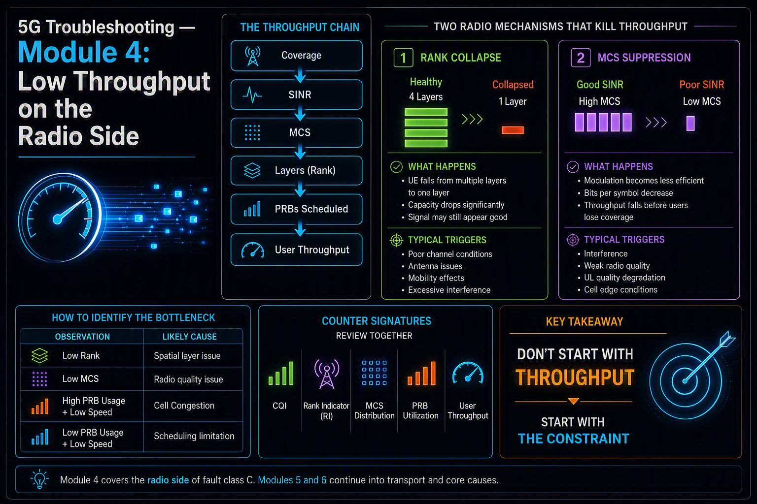
A 5G low throughput complaint is the most commonly misdiagnosed fault in the network, and the reason is organizational rather than technical. Throughput is the KPI radio teams own, so a throughput ticket lands on a radio engineer’s desk regardless of where the constraint actually sits. That engineer opens the radio dashboards, finds something imperfect, and optimizes it. Sometimes throughput improves. Often it does not, and nobody can say why.
This module covers the radio half of fault class C. It gives you the chain that determines throughput, the specific counter pairs that identify which link in that chain is the constraint, and the two mechanisms that get misread more than any others: rank collapse, and outer-loop MCS suppression. Modules 5 and 6 continue into transport and core causes.
Optimizing a stage that was never the constraint is the most common way to spend a week and change nothing.
In this module
- Part 1 — What actually limits 5G low throughput
- Part 2 — Establish the ceiling before you measure anything
- Part 3 — Rank: the most misread number in the cell
- Part 4 — CQI, MCS and the outer loop
- Part 5 — HARQ retransmission and what it really tells you
- Part 6 — 5G low throughput: link problem or scheduling problem
- Part 7 — Uplink is a separate investigation
- Part 8 — Counters and vendor mapping
- Part 9 — Worked example
- Part 10 — The full decision tree
Part 1 — What actually limits 5G low throughput
Throughput is not a single quantity that a single thing degrades. It is the product of five stages, and because they multiply, the smallest one sets the ceiling for all of them. Doubling a stage that was not the constraint changes nothing at all.
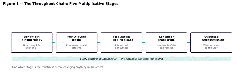
Figure 1 — the five stages that determine throughput. Because they multiply, only the smallest matters until you fix it.
| Stage | Determines | Fails because of |
| Bandwidth × numerology | Total resource elements available | Configuration — carrier not deployed, or a narrower BWP than assumed |
| MIMO layers (rank) | Parallel streams to this UE | Spatial conditions, antenna correlation, UE capability |
| Modulation and coding | Bits carried per symbol | SINR, and the outer loop reacting to BLER |
| Scheduler share | PRBs this UE receives | Cell load, QoS priority, competing traffic |
| Overhead and retransmission | What survives to the application | HARQ retransmission, RLC, protocol overhead |
The practical consequence is that the first question in any throughput investigation is not “what looks bad” but “which stage is the constraint.” A cell with excellent SINR and rank 4 will still deliver poor throughput if the UE is scheduled on 8 PRBs out of 273. A cell with 80 percent PRB allocation to one UE will still deliver poor throughput if the MCS is 4.
Throughput is multiplicative. Improving anything except the smallest stage produces no change the user can feel.
Part 2 — Establish the ceiling before you measure anything
Before comparing a cell against its neighbors or against a target, work out what the configuration can actually deliver. A surprising share of throughput tickets resolve here, before any radio analysis at all.
The four things to confirm
- Channel bandwidth and numerology as configured, not as planned. A 100 MHz plan running on a 60 MHz carrier because the rest of the spectrum was not cleared is a common finding, and no radio work will recover the difference.
- The TDD pattern. A downlink-heavy pattern and a balanced pattern deliver very different downlink ceilings from identical spectrum, and a UE tested on a cell configured for uplink-favorable operation will underperform for reasons that have nothing to do with the link.
- UE capability. Check the reported category, supported layers and supported modulation. A device limited to two layers or to 64QAM cannot reach a figure calculated for four layers and 256QAM regardless of conditions.
- Subscribed session-AMBR and UE-AMBR. If throughput plateaus at a suspiciously round number — exactly 50, exactly 100 — this is almost always why, and it is a policy setting rather than a radio one.
That last check deserves emphasis because of how it presents. An AMBR ceiling produces a perfectly flat throughput curve regardless of radio conditions, which looks like an unusually stable link rather than a limit. Engineers frequently interpret it as a good result.
The bandwidth and numerology relationship is worth understanding properly rather than looking up, because it determines the ceiling for everything else — spectrum bands and why they matter covers FR1 and FR2 allocation, and NR frame structure and slot-based scheduling covers how numerology and the TDD pattern translate into usable capacity.
Part 3 — Rank: the most misread number in the cell
Rank is the number of independent spatial streams the network can send to a UE simultaneously. Rank 2 is twice the theoretical throughput of rank 1 at the same MCS. It is therefore one of the highest-leverage numbers in the cell, and it is routinely misinterpreted.
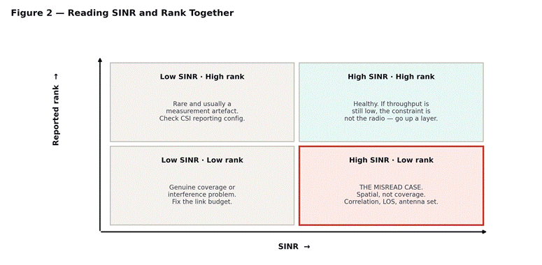
Figure 2 — SINR and rank must be read together. The bottom-right quadrant is where most misdiagnosis happens.
Why the bottom-right quadrant matters
Good SINR with low rank is the case engineers get wrong. The instinct is that poor throughput with poor rank means poor coverage, so the response is a tilt change or a power increase. But rank is not determined by signal strength. It is determined by whether the propagation environment provides enough spatial separation for the antenna array to distinguish independent streams.
Three conditions collapse rank while leaving SINR untouched:
- Strong line of sight. A clean, dominant path is excellent for SINR and terrible for spatial multiplexing, because every antenna element sees essentially the same channel. Rooftop-to-rooftop fixed wireless links frequently show this.
- Antenna correlation at the UE. A device holding its two antennas in close proximity, or held in a way that shadows one, cannot resolve two streams even in a rich scattering environment.
- A degraded or misconfigured antenna set at the gNB. A failed radio branch, or a beam configuration that does not deliver the spatial diversity the planner assumed, caps rank across the whole cell rather than for one UE.
The diagnostic distinction is straightforward once you look for it. If rank is low across every UE in the cell, suspect the gNB antenna set or the propagation environment. If rank is low for specific UEs while others achieve rank 3 or 4 in the same cell at similar SINR, suspect device behavior.
The mechanics of how spatial layers are constructed, and why the scattering environment rather than the link budget governs them, are covered in massive MIMO and beamforming. It is worth reading before making any tilt change intended to recover rank, because tilt changes usually will not.
Checking rank properly
- Look at the rank distribution, not the average. An average of 2.1 could be a cell where everything reports 2, or one where half report 1 and half report 3. Those are different problems.
- Correlate rank against SINR across the cell. A cloud that shows high SINR with rank 1 confirms the spatial diagnosis rather than the coverage one.
- Check whether rank is capped by the configured maximum layers rather than by conditions. A cell configured for two layers will never report four however good the environment.
- Compare against a neighboring cell with the same hardware and a different environment. If both show identical rank distributions, the constraint is configuration; if they differ, it is environmental.
Part 4 — CQI, MCS and the outer loop
The second high-leverage stage is modulation and coding. It is governed by two nested control loops, and the interaction between them explains the single most confusing symptom in radio troubleshooting: an MCS that has collapsed while SINR looks entirely healthy.
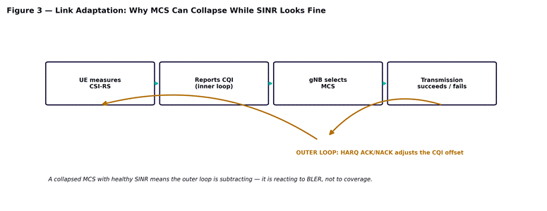
Figure 3 — the inner loop reports channel quality; the outer loop corrects it based on actual outcomes.
How the two loops interact
The inner loop is the UE’s own report. It measures CSI-RS, estimates what modulation and coding it could decode at the target error rate, and reports a CQI. The gNB maps that to an MCS.
The outer loop sits on top and does not trust the report. It watches HARQ acknowledgements, and when the actual block error rate exceeds the configured target, it subtracts an offset from the reported CQI before mapping to MCS. When transmissions succeed more than expected, it adds. Over time the offset converges on whatever correction that particular UE, in that particular environment, actually needs.
This is the mechanism behind the confusing case. If the UE consistently over-reports its capability — because of interference that fluctuates faster than the reporting period, or because of an optimistic implementation — the outer loop learns to subtract a large offset. The result is a low MCS alongside a high SINR, and no amount of coverage improvement will change it, because the loop is reacting to decoding failures rather than to signal strength.
| Symptom | Mechanism | What to do |
| Low MCS, low SINR | Working as intended | Fix the link budget — this is genuine coverage |
| Low MCS, high SINR | Outer loop subtracting on BLER | Look for fast-fading interference or UE over-reporting |
| MCS oscillating widely | Loop unable to converge | Unstable interference; check for intermittent sources |
| MCS capped below maximum | Configuration limit | Check the configured maximum MCS and modulation order |
One practical note on the second row. The outer loop is doing the right thing — it is protecting throughput by preventing repeated retransmission. The fault is not the loop; it is whatever is causing the UE’s reports to be unreliable. Disabling or clamping the outer loop to force a higher MCS almost always makes throughput worse, because the retransmissions cost more than the higher modulation gains.
A collapsed MCS with healthy SINR is the outer loop protecting you from something. Find what it is reacting to rather than overriding it.
Part 5 — HARQ retransmission and what it really tells you
HARQ retransmission rate is one of the most useful counters in a throughput investigation and one of the most frequently misread, because a low number is not automatically good.
Link adaptation targets a specific initial block error rate — commonly around ten percent. That target is deliberate. It represents the point at which the throughput gained by transmitting aggressively exceeds the throughput lost to retransmitting the failures. A system running at one percent BLER is not performing well; it is being too conservative and leaving capacity unused.
| Observed BLER | Interpretation | Action |
| Around target (~10%) | Link adaptation working correctly | Nothing — look elsewhere for the constraint |
| Well below target | Excessively conservative | Check the outer loop offset and the BLER target itself |
| Well above target | Adaptation cannot keep up | Fast fading, high mobility, or unstable interference |
| High with high MCS | Aggressive assignment | Outer loop has not converged, or the target is misconfigured |
The row that matters most for diagnosis is the third. Sustained BLER above target means the channel is changing faster than the reporting and adaptation cycle can track. That happens at high speed, under rapidly varying interference, or when the CSI reporting period is configured too long for the environment. The fix is in reporting configuration or interference management, not in coverage.
The retransmission mechanism itself — soft combining, incremental redundancy, and why a failed transmission is not wasted — carries over from LTE and is worth understanding before interpreting these counters. See HARQ and how retransmission extracts value from failed attempts.
Part 6 — 5G low throughput: link problem or scheduling problem
Every 5G low throughput investigation eventually resolves into one of two categories, and they have almost nothing in common. A link problem means the PRBs the UE receives carry too little. A scheduling problem means the PRBs carry plenty and the UE receives too few of them.
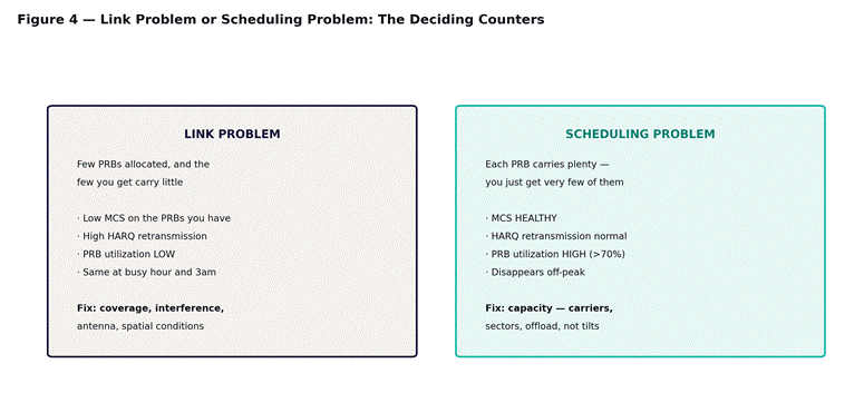
Figure 4 — the counter signatures that separate a link problem from a scheduling problem.
The deciding counter is PRB utilization
If cell PRB utilization is high — above roughly seventy percent at the times throughput is poor — the cell is running out of resources and the scheduler is dividing them. Every UE gets a small share. This is a capacity problem, and the fixes are capacity fixes: additional carriers, additional sectors, traffic offload, or in some cases QoS reprioritization to protect specific traffic.
If PRB utilization is low and throughput is still poor, the scheduler is offering resources the link cannot use well. This is a link problem, and the fixes are the ones covered in Parts 3 through 5. Note that in a disaggregated RAN the scheduler lives in the DU, so a scheduling problem is diagnosed on a different physical element from a coverage one — see the CU/DU/RU split.
The time test
A second discriminator, and often faster than pulling counters: does the problem disappear off-peak? A scheduling problem is load-dependent by definition and largely vanishes at three in the morning. A link problem does not care what time it is. If a customer reports poor throughput at all hours and PRB utilization is moderate, you can rule out congestion before opening a single dashboard.
The case that looks like both
One combination causes genuine confusion: moderate PRB utilization with poor throughput and a healthy MCS. This is usually scheduler configuration rather than either category — a proportional fair scheduler weighting against this UE, a QoS profile with low priority, or a guaranteed bit rate commitment to other traffic consuming capacity that appears available. Check the QoS flow the traffic actually mapped to before concluding anything.
Scheduler behavior is governed by the QoS parameters attached to each flow, so a throughput problem confined to one traffic type or one enterprise customer is very often a policy question rather than a radio one — QoS and 5QI covers the standardized table and what each parameter actually controls, and network slicing covers slice-level resource commitments that can cap a cell’s available capacity before any UE is scheduled.
Part 7 — Uplink is a separate investigation
Almost everything above concerns the downlink. Uplink throughput fails for related but distinct reasons, and treating them as one investigation produces wrong conclusions.
| Constraint | Why it differs from downlink | Signature |
| UE transmit power | The UE has a fraction of the gNB’s power budget | Degrades sharply with distance while downlink holds up |
| TDD pattern | Uplink slots are usually the minority allocation | Hard ceiling regardless of conditions |
| No massive MIMO gain | Array gain is largely a downlink benefit | Uplink range far shorter than downlink coverage suggests |
| Waveform | Transform precoding trades peak rate for coverage | Lower peak throughput at cell edge by design |
The practical consequence is the uplink-downlink imbalance that appears throughout this course. A UE can measure an excellent downlink on a cell whose uplink it cannot reach usably. That produces poor uplink throughput, failed random access, and in non-standalone deployments the SCG failures covered in Module 3 — all from the same underlying cause, all presenting differently.
The access-side consequences of the same imbalance are covered in NR initial access — cell search, SSB and random access, and the preamble planning that governs whether the uplink attempt succeeds at all in RACH preamble planning.
Part 8 — Counters and vendor mapping
As in the earlier modules, the measurement points are defined by the protocol and are identical across vendors; only the counter names differ.
| 3GPP TS 28.552 reference | Measures | Read it against |
| DRB.UEThpDl / .UEThpUl | Per-UE throughput | The calculated ceiling from Part 2, not a neighbor cell |
| RRU.PrbUsedDl / .PrbTotDl | PRB utilization | Throughput — this pair decides link vs scheduling |
| CARR.AverageLayersDl | Average spatial layers | SINR distribution — the Figure 2 matrix |
| MAC.DlHarqFail / total | HARQ failure rate | The configured BLER target, not against zero |
| CQI distribution | Reported channel quality | The resulting MCS — a gap between them is the outer loop |
| Measurement point | Huawei (MAE-Access) | Ericsson (ENM) |
| Downlink throughput | N.ThpVol.DL domain counters | pm-prefixed PDCP volume and time counters |
| PRB utilization | N.PRB.DL.Used.Avg style naming | pm-prefixed PRB usage counters |
| Spatial layers | N.MIMO domain counters | pm-prefixed MIMO layer distribution |
The same caution applies as in Modules 2 and 3: Huawei’s N.<Domain>.<Metric> convention and Ericsson’s pm prefix are reliable, but confirm the exact strings against the PM counter reference for your own software baseline before building a report on them. Throughput counters in particular vary in whether they measure PDCP or MAC layer volume, and whether they exclude time when the UE had no data to send — two definitions that produce very different numbers from the same traffic.
A throughput counter that excludes idle time and one that does not will disagree by a factor of several. Know which yours is before comparing anything.
Part 9 — Worked example
An enterprise customer on a dedicated indoor system reports downlink throughput of roughly 90 Mbps against an expectation of 400. The system is 100 MHz, four-layer capable, and the customer’s devices are current flagship handsets. RSRP throughout the building is better than -75 dBm and SINR is consistently above 25 dB — conditions that look close to ideal.
Part 2 first. The configuration is confirmed at 100 MHz with a downlink-favorable TDD pattern, the devices support four layers and 256QAM, and the session-AMBR is set well above the observed figure. The ceiling is genuinely around 400 Mbps, so the expectation is reasonable.
Part 3 next. Average reported rank is 1.1. Almost every UE in the building is reporting rank 1 despite excellent SINR — the bottom-right quadrant of Figure 2. The instinct at this point is to conclude something is wrong with coverage, but SINR at 25 dB rules that out definitively.
Part 4 and 5 come back clean. MCS is high, consistent with the reported SINR, and HARQ retransmission sits close to the ten percent target. The link is carrying as much per layer as it should. There is simply only one layer.
Part 6 rules out scheduling: PRB utilization is under twenty percent, and the problem is identical at three in the morning.
So the constraint is rank, and rank alone. The mechanism is the indoor system’s antenna design — a distributed system where each antenna carries the same signal provides excellent coverage and no spatial diversity whatsoever. Every antenna element presents the UE with essentially the same channel, so the array cannot resolve independent streams. The customer is getting exactly the throughput a single-layer system delivers, because that is what was installed.
The fix is not a radio parameter. It requires either a different antenna configuration capable of genuine spatial separation, or a revised expectation set with the customer. Two rounds of power and tilt optimization would have achieved nothing, and on a distributed indoor system there is not much tilt to adjust in the first place.
Part 10 — The full decision tree
Step 1 — Calculate the ceiling
- Confirm bandwidth, numerology and TDD pattern as configured, not as designed.
- Confirm UE capability — layers and modulation order.
- Check session-AMBR and UE-AMBR. A flat curve at a round number is a policy limit, not a radio result.
- Compare observed throughput against that calculated ceiling, never against a neighboring cell.
Step 2 — Link or scheduling
- Check PRB utilization at the times throughput is poor. Above roughly seventy percent means capacity; below means link.
- Apply the time test — does the problem disappear off-peak? If yes, it is load, whatever the counters suggest.
- If PRB utilization is moderate and MCS is healthy, check the QoS flow and scheduler weighting before continuing.
Step 3 — If it is a link problem, work the stages
- Rank first — it is the largest single multiplier. Read rank and SINR together using the Figure 2 matrix.
- Then MCS — compare the reported CQI against the assigned MCS. A gap means the outer loop is correcting.
- Then HARQ — compare against the configured BLER target, not against zero.
- Check the downlink and uplink separately. They fail for different reasons and one can be healthy while the other is not.
Step 4 — Change one thing
- Identify the specific stage that is the constraint and state it explicitly before making any change.
- Change one parameter, then re-measure over at least a full busy hour.
- Confirm against the customer’s original measurement, not against the counter you changed.
What comes next
Module 5 takes the transport side of fault class C — interface negotiation, MTU and fragmentation on the GTP-U path, latency and its effect on TCP window behavior, and packet loss. Module 6 covers the core and policy side. If you need the underlying architecture, the 14-module Introduction to 5G course covers the air interface and core design this course assumes.